- Import Data and Packages
import numpy as np
import pandas as pd
import seaborn as sns
import matplotlib.pyplot as plt
import os
print(os.listdir("../input"))
import warnings
warnings.filterwarnings("ignore")
['WA_Fn-UseC_-Telco-Customer-Churn.csv']
df = pd.read_csv("../input/WA_Fn-UseC_-Telco-Customer-Churn.csv",na_values = [" "])
df.head()
| customerID | gender | SeniorCitizen | Partner | Dependents | tenure | PhoneService | MultipleLines | InternetService | OnlineSecurity | OnlineBackup | DeviceProtection | TechSupport | StreamingTV | StreamingMovies | Contract | PaperlessBilling | PaymentMethod | MonthlyCharges | TotalCharges | Churn | |
|---|---|---|---|---|---|---|---|---|---|---|---|---|---|---|---|---|---|---|---|---|---|
| 0 | 7590-VHVEG | Female | 0 | Yes | No | 1 | No | No phone service | DSL | No | Yes | No | No | No | No | Month-to-month | Yes | Electronic check | 29.85 | 29.85 | No |
| 1 | 5575-GNVDE | Male | 0 | No | No | 34 | Yes | No | DSL | Yes | No | Yes | No | No | No | One year | No | Mailed check | 56.95 | 1889.50 | No |
| 2 | 3668-QPYBK | Male | 0 | No | No | 2 | Yes | No | DSL | Yes | Yes | No | No | No | No | Month-to-month | Yes | Mailed check | 53.85 | 108.15 | Yes |
| 3 | 7795-CFOCW | Male | 0 | No | No | 45 | No | No phone service | DSL | Yes | No | Yes | Yes | No | No | One year | No | Bank transfer (automatic) | 42.30 | 1840.75 | No |
| 4 | 9237-HQITU | Female | 0 | No | No | 2 | Yes | No | Fiber optic | No | No | No | No | No | No | Month-to-month | Yes | Electronic check | 70.70 | 151.65 | Yes |
# check NA
df.isna().sum()
customerID           0
gender               0
SeniorCitizen        0
Partner              0
Dependents           0
tenure               0
PhoneService         0
MultipleLines        0
InternetService      0
OnlineSecurity       0
OnlineBackup         0
DeviceProtection     0
TechSupport          0
StreamingTV          0
StreamingMovies      0
Contract             0
PaperlessBilling     0
PaymentMethod        0
MonthlyCharges       0
TotalCharges        11
Churn                0
dtype: int64
# drop NA
df = df.dropna()
2.Data Analytic
# drop customerID and churn to make train dataset
customerID = df["customerID"]
Churn = df["Churn"]
df = df.drop(["customerID","Churn"],axis = 1)
# change data type :
df["SeniorCitizen"] = df["SeniorCitizen"].astype("object")

print(df.dtypes)
gender               object
SeniorCitizen        object
Partner              object
Dependents           object
tenure                int64
PhoneService         object
MultipleLines        object
InternetService      object
OnlineSecurity       object
OnlineBackup         object
DeviceProtection     object
TechSupport          object
StreamingTV          object
StreamingMovies      object
Contract             object
PaperlessBilling     object
PaymentMethod        object
MonthlyCharges      float64
TotalCharges        float64
dtype: object
Usually, Customer churn problem is a imbalanced problem. For the data with less than 20% Churn rate, I will consider use “ROC_AUC” as metric. While in this case, Churn rate is 26%, so I will use “accuracy” as metric here.
- When there is a modest class imbalance like 4:1 in the example above it can cause problems.
- From https://machinelearningmastery.com/tactics-to-combat-imbalanced-classes-in-your-machine-learning-datasets
# Churn Rate
print(Churn.value_counts())
print("-"*40)
print("Churn Rate", sum(Churn == "Yes")/len(Churn))
No     5163
Yes    1869
Name: Churn, dtype: int64
----------------------------------------
Churn Rate 0.26578498293515357
# plot numeric values
_,ax = plt.subplots(3,1,figsize = (9,9))
for i,c in enumerate(df.select_dtypes([np.number]).columns) :
    # print(i,c)
    sns.distplot(df[c],ax = ax[i])
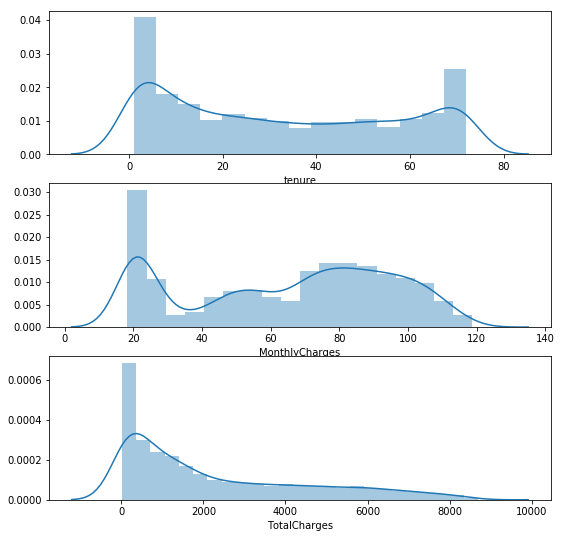
Many of Numeric values are 0 and skewness is high. Considering Scale values.
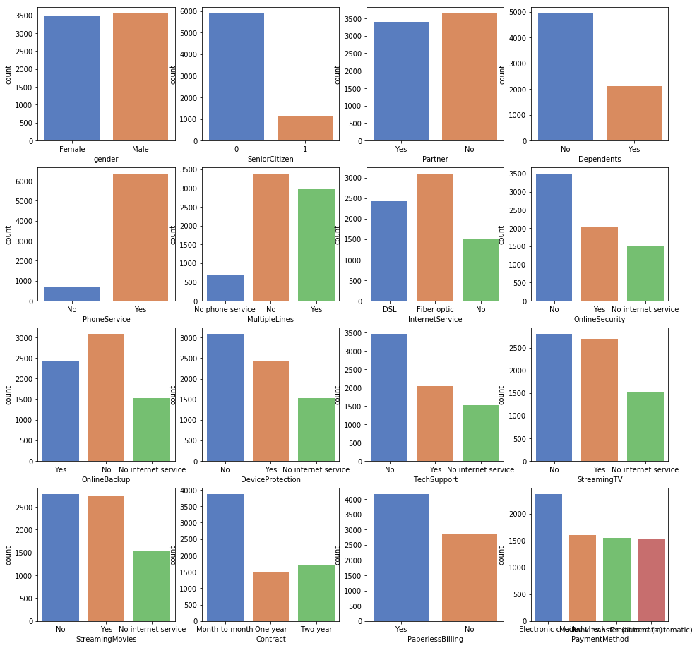
Plot all categorical variables
_,ax = plt.subplots(4,4,figsize = (16,16))
for i in range(0,4) :
    for j in range(0,4) :
        sns.countplot(df.select_dtypes(exclude=["number"]).iloc[:,4*i+j],ax = ax[i,j],palette = "muted")
3.Data preprocessing
# pipeline with scale / onehotencoder / with LR classfication as baseline model
from sklearn.preprocessing import OneHotEncoder,StandardScaler
from sklearn.pipeline import Pipeline
from sklearn.linear_model import LogisticRegression


df_dummies = pd.get_dummies(df)

# train test split
from sklearn.model_selection import train_test_split

x_train,x_test,y_train,y_test = train_test_split(df_dummies,Churn,test_size = 0.25,random_state = 1)
4.Baseline Modeling
# baseline model with Logistic Regression
from sklearn.model_selection import cross_val_score,KFold

cv =  KFold(10,random_state=1)
baseline = LogisticRegression(random_state = 1)
baseline.fit(x_train,y_train)
cv_bl = cross_val_score(baseline,x_test,y_test,cv =cv).mean()

#bl_pred = baseline.predict(x_test)
print("Baseline model accuracy is :",cv_bl) # 0.8048993506493506
Baseline model accuracy is : 0.8048993506493506
5.Feature engineering
- Categorical vs Churn
_,ax = plt.subplots(4,4,figsize = (16,16))
for i in range(0,4) :
    for j in range(0,4) :
        sns.countplot(df.select_dtypes(exclude=["number"]).iloc[:,4*i+j],ax = ax[i,j],palette = "muted",hue = Churn,dodge = False)
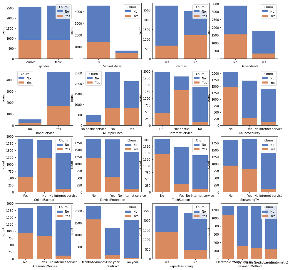
What we know :
1.Senior are more possible to lose compared to junor citizen
2.Single ppl are more possible to lose compared the one with panter
3.Independent ppl are mroe possible to lose compared the one who relies on another
4.Ppl with no internet service are more possible to be loyalty maybe because they have less methods to get more new info.
5.Pple with OnlineSecurity, OnlineBackup, OnlineProtection, Deviceprotection,TechSupport are more likely to be loyalty.
6.Ppl with more than 1 year contract are more likely to be loyalty and longer the contract, less the churn.
7.Ppl with paperbilling are more likely to be loyalt customer.
8.More ppl in E-billing payment method are lost.
_,ax = plt.subplots(3,1,figsize = (9,12))
for i,c in enumerate(df.select_dtypes([np.number]).columns) :
    # print(i,c)
    sns.boxplot(x = df[c],y = Churn,ax = ax[i],palette = "muted")
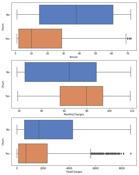
1.Low tensure and high monthly charge customer more likely to lose.
2.Low total charge clients more likely to lose while there are many outliers.
3.There are some clients whose TotalCharges are equal to monthcharges, which means they use service for only 1 month or they spend 0 in other months.
# short term
df["Short_term"] =  (df.TotalCharges == df.MonthlyCharges).astype('object')
sns.countplot(df["Short_term"],palette = "muted",hue = Churn,dodge = False)
<matplotlib.axes.subplots.AxesSubplot at 0x7f832e541940>
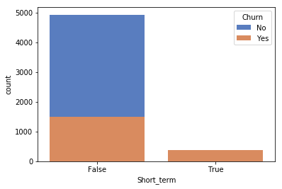
All short-term clients are Churn customer.
Check out month stay with churn
# how many month they stay here
df["Month_Stay"] = df.TotalCharges/df.MonthlyCharges
sns.boxplot(y =df["Month_Stay"] ,x = Churn,palette = "muted")
<matplotlib.axes.subplots.AxesSubplot at 0x7f832e1b9a20>
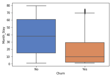
Lower month stay will definetely lead to more churn
df["long_contract_no_internet"] = ((df.Contract == "Two year") & (df.InternetService == "No")).astype("object")
sns.countplot(df["long_contract_no_internet"],palette = "muted",hue = Churn,dodge = False)
<matplotlib.axes.subplots.AxesSubplot at 0x7f832d9afd30>
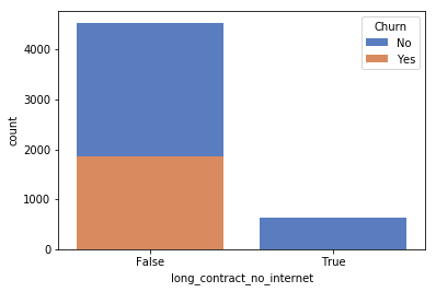
All long_contract_no_internet are loyalty customer
6.Modeling
df = pd.get_dummies(df) # get k-1 dummies
x_train,x_test,y_train,y_test = train_test_split(df,Churn,test_size = 0.25,random_state = 1)
from sklearn.ensemble import GradientBoostingClassifier,RandomForestClassifier
from sklearn.tree import DecisionTreeClassifier
import lightgbm as lgb
from sklearn.neighbors import KNeighborsClassifier

# all algorithms I want to use
algorithms = pd.DataFrame({
    "Name" : ["Logistic Regression","Random Forest","GBM","DTree","LGBM","KNN"],
    "Algorithm" : [LogisticRegression(random_state=1),RandomForestClassifier(random_state = 1),
                   GradientBoostingClassifier(random_state=1),DecisionTreeClassifier(random_state=1),
                   lgb.LGBMClassifier(random_state=1),KNeighborsClassifier()]
})
# default score with default parameters
from sklearn.feature_selection import SelectKBest

score = []
for i in range(1,len(algorithms)+1) :
    clf = Pipeline([
        ("featureselection",SelectKBest(k = x_train.shape[1])),
        (algorithms.Name[i-1],algorithms.Algorithm[i-1])
    ])
    clf.fit(x_train,y_train)
    score.append(cross_val_score(clf,x_test,y_test,cv = cv).mean())
    #print("{} accuracy is {}:".format(algorithms.Name[i-1],(pred == y_test).mean()))
algorithms["Score"] = score
algorithms
| Name | Algorithm | Score | |
|---|---|---|---|
| 0 | Logistic Regression | LogisticRegression(C=1.0, class_weight=None, d... | 0.804899 |
| 1 | Random Forest | (DecisionTreeClassifier(class_weight=None, cri... | 0.778149 |
| 2 | GBM | ([DecisionTreeRegressor(criterion='friedman_ms... | 0.785000 |
| 3 | DTree | DecisionTreeClassifier(class_weight=None, crit... | 0.732091 |
| 4 | LGBM | LGBMClassifier(boosting_type='gbdt', class_wei... | 0.782714 |
| 5 | KNN | KNeighborsClassifier(algorithm='auto', leaf_si... | 0.761666 |
7.Parameter tuning
- Logistic Regression
# feature selection for LR
lr_score = []
for i in np.arange(0.5,1.5,0.2) :
    for j in range(20,x_train.shape[1]+1) :
        clf = Pipeline([
                ("featureselection",SelectKBest(k = j)),
                ("LR",LogisticRegression(random_state=1,C = i))])
        clf.fit(x_train,y_train)
        cvs = cross_val_score(clf,x_test,y_test,cv = cv).mean()
        lr_score.append(cvs)
        #print("Score is {} with C = {} and {} feature".format(cvs,i,j))
print("Best Score is {}".format(max(lr_score)))
# Score is 0.8157077922077922 with C = 1.3 and 31 feature
Best Score is 0.8157077922077922
from sklearn.metrics import classification_report,confusion_matrix
clf_lr = Pipeline([
                ("featureselection",SelectKBest(k = 31)),
                ("LR",LogisticRegression(random_state=1,C = 1.3))])
pred = clf_lr.fit(x_train,y_train).predict(x_test)
print(classification_report(y_test,pred))
sns.heatmap(confusion_matrix(y_test,pred),annot=True,cmap = "PuBuGn")
              precision    recall  f1-score   support

          No       0.84      0.90      0.87      1294
         Yes       0.66      0.54      0.59       464

   micro avg       0.81      0.81      0.81      1758
   macro avg       0.75      0.72      0.73      1758
weighted avg       0.80      0.81      0.80      1758


<matplotlib.axes.subplots.AxesSubplot at 0x7f834414f2b0>
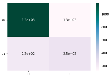
TPR for “YES” is 0.54, not so good. We have a really bad guess on churn = “yes”.
- GBM
# parameter tuning in GBM
# default value is 0.785000

from sklearn.model_selection import GridSearchCV
clf_pl = Pipeline([
                ("featureselection",SelectKBest(k = x_train.shape[1])),
                ("GBM",GradientBoostingClassifier(random_state=1))])
param = {
    "GBM__learning_rate" : np.arange(0.06,0.08,0.01),
    "GBM__n_estimators" : range(59,63,2),
    'GBM__max_depth':range(6,8,1),
    'GBM__min_samples_split':range(485,511,5),
    "GBM__subsample": [0.8]
}
clf_gbm = GridSearchCV(clf_pl,param,cv = cv,n_jobs = -1,verbose = 1)
clf_gbm.fit(x_train,y_train)
print(clf_gbm.best_params_)
print("-"*40)
print("Best Score is {}".format(clf_gbm.best_score_)) # 0.8103905953735305
Fitting 10 folds for each of 72 candidates, totalling 720 fits


[Parallel(n_jobs=-1)]: Using backend LokyBackend with 4 concurrent workers.
[Parallel(n_jobs=-1)]: Done  42 tasks      | elapsed:   23.8s
[Parallel(n_jobs=-1)]: Done 192 tasks      | elapsed:  1.4min
[Parallel(n_jobs=-1)]: Done 442 tasks      | elapsed:  3.0min
[Parallel(n_jobs=-1)]: Done 720 out of 720 | elapsed:  4.8min finished


{'GBM__learning_rate': 0.06999999999999999, 'GBM__max_depth': 7, 'GBM__min_samples_split': 495, 'GBM__n_estimators': 59, 'GBM__subsample': 0.8}
----------------------------------------
Best Score is 0.8088737201365188
gbm = GradientBoostingClassifier(random_state=1,learning_rate=0.07,max_depth=7,min_samples_split=495,n_estimators=59,subsample=0.8)
pred = gbm.fit(x_train,y_train).predict(x_test)
print(classification_report(y_test,pred))
sns.heatmap(confusion_matrix(y_test,pred),annot=True,cmap = "PuBuGn")
              precision    recall  f1-score   support

          No       0.83      0.91      0.87      1294
         Yes       0.66      0.48      0.56       464

   micro avg       0.80      0.80      0.80      1758
   macro avg       0.75      0.70      0.71      1758
weighted avg       0.79      0.80      0.79      1758


<matplotlib.axes.subplots.AxesSubplot at 0x7f833c769f98>
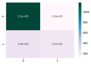
GBM have a better estimate on Churn = “No” while bad on Yes
- Decision Tree
# 0.732091
clf_dt = Pipeline([
                ("featureselection",SelectKBest(k = x_train.shape[1])),
                ("DTree",DecisionTreeClassifier(random_state=1))])
param = {
    "DTree__criterion": ["gini","entropy"],
    "DTree__max_depth" :range(4,9),
    "DTree__min_samples_split":np.arange(0.1,0.6,0.1),
    "DTree__min_samples_leaf":np.arange(0.1,0.5,0.1),
    #"DTree__max_features " : ["auto","log2","sqrt"],
    "DTree__class_weight" : ["balanced",None]
}
clf_dt = GridSearchCV(clf_dt,param,cv = cv,n_jobs = -1,verbose = 1)
clf_dt.fit(x_train,y_train)
print(clf_dt.best_params_)
print("-"*40)
print("Best Score is {}".format(clf_dt.best_score_)) # 0.7897231702692453
Fitting 10 folds for each of 400 candidates, totalling 4000 fits


[Parallel(n_jobs=-1)]: Using backend LokyBackend with 4 concurrent workers.
[Parallel(n_jobs=-1)]: Done  76 tasks      | elapsed:    1.3s
[Parallel(n_jobs=-1)]: Done 376 tasks      | elapsed:    6.3s
[Parallel(n_jobs=-1)]: Done 876 tasks      | elapsed:   14.7s
[Parallel(n_jobs=-1)]: Done 1576 tasks      | elapsed:   26.6s
[Parallel(n_jobs=-1)]: Done 2476 tasks      | elapsed:   42.2s
[Parallel(n_jobs=-1)]: Done 3576 tasks      | elapsed:   59.3s


{'DTree__class_weight': None, 'DTree__criterion': 'gini', 'DTree__max_depth': 4, 'DTree__min_samples_leaf': 0.1, 'DTree__min_samples_split': 0.1}
----------------------------------------
Best Score is 0.7897231702692453


[Parallel(n_jobs=-1)]: Done 4000 out of 4000 | elapsed:  1.1min finished
import graphviz
from sklearn.tree import export_graphviz
dt = DecisionTreeClassifier(random_state=1,criterion="gini",max_depth=4,min_samples_leaf=0.1,min_samples_split=0.1)
dt.fit(x_train,y_train)
dot_data = export_graphviz(dt, out_file=None,
                         feature_names=x_train.columns,
                         class_names=y_train,
                         filled=True, rounded=True,
                         special_characters=True)
graph = graphviz.Source(dot_data)
graph

Tuned_Score = [0.8157077922077922,0,0.8088737201365188,0.7897231702692453,0,0]
algorithms["Tuned Score"] = Tuned_Score
algorithms
| Name | Algorithm | Score | Tuned Score | |
|---|---|---|---|---|
| 0 | Logistic Regression | LogisticRegression(C=1.0, class_weight=None, d... | 0.804899 | 0.815708 |
| 1 | Random Forest | (DecisionTreeClassifier(class_weight=None, cri... | 0.778149 | 0.000000 |
| 2 | GBM | ([DecisionTreeRegressor(criterion='friedman_ms... | 0.785000 | 0.808874 |
| 3 | DTree | DecisionTreeClassifier(class_weight=None, crit... | 0.732091 | 0.789723 |
| 4 | LGBM | LGBMClassifier(boosting_type='gbdt', class_wei... | 0.782714 | 0.000000 |
| 5 | KNN | KNeighborsClassifier(algorithm='auto', leaf_si... | 0.761666 | 0.000000 |
For Furture Study :
- Deep analysis in Churn = “Yes”
- Feature engineering
- Normalized numeric data or categorical numeric data
- Using Ensembling Algorithms to combine some simple algorithms