This Wine data set contains the results of a chemical analysis of wines grown in a specific area of Italy. I use KMeans Algorithm to cluster different Wine and check if the result is correct by comparing with label variable.
@author: Ha
1.Import package and data
import numpy as np # linear algebra
import pandas as pd # data processing, CSV file I/O (e.g. pd.read_csv)
import seaborn as sns
import matplotlib.pyplot as plt

import os
print(os.listdir("../input"))
['Wine.csv']
df = pd.read_csv("../input/Wine.csv")
df.head()
| Alcohol | Malic_Acid | Ash | Ash_Alcanity | Magnesium | Total_Phenols | Flavanoids | Nonflavanoid_Phenols | Proanthocyanins | Color_Intensity | Hue | OD280 | Proline | Customer_Segment | |
|---|---|---|---|---|---|---|---|---|---|---|---|---|---|---|
| 0 | 14.23 | 1.71 | 2.43 | 15.6 | 127 | 2.80 | 3.06 | 0.28 | 2.29 | 5.64 | 1.04 | 3.92 | 1065 | 1 |
| 1 | 13.20 | 1.78 | 2.14 | 11.2 | 100 | 2.65 | 2.76 | 0.26 | 1.28 | 4.38 | 1.05 | 3.40 | 1050 | 1 |
| 2 | 13.16 | 2.36 | 2.67 | 18.6 | 101 | 2.80 | 3.24 | 0.30 | 2.81 | 5.68 | 1.03 | 3.17 | 1185 | 1 |
| 3 | 14.37 | 1.95 | 2.50 | 16.8 | 113 | 3.85 | 3.49 | 0.24 | 2.18 | 7.80 | 0.86 | 3.45 | 1480 | 1 |
| 4 | 13.24 | 2.59 | 2.87 | 21.0 | 118 | 2.80 | 2.69 | 0.39 | 1.82 | 4.32 | 1.04 | 2.93 | 735 | 1 |
2.Basic Data Information
# drop Customer_Segment
label = df.Customer_Segment
df = df.drop("Customer_Segment",axis = 1)
df.describe()
| Alcohol | Malic_Acid | Ash | Ash_Alcanity | Magnesium | Total_Phenols | Flavanoids | Nonflavanoid_Phenols | Proanthocyanins | Color_Intensity | Hue | OD280 | Proline | |
|---|---|---|---|---|---|---|---|---|---|---|---|---|---|
| count | 178.000000 | 178.000000 | 178.000000 | 178.000000 | 178.000000 | 178.000000 | 178.000000 | 178.000000 | 178.000000 | 178.000000 | 178.000000 | 178.000000 | 178.000000 |
| mean | 13.000618 | 2.336348 | 2.366517 | 19.494944 | 99.741573 | 2.295112 | 2.029270 | 0.361854 | 1.590899 | 5.058090 | 0.957449 | 2.611685 | 746.893258 |
| std | 0.811827 | 1.117146 | 0.274344 | 3.339564 | 14.282484 | 0.625851 | 0.998859 | 0.124453 | 0.572359 | 2.318286 | 0.228572 | 0.709990 | 314.907474 |
| min | 11.030000 | 0.740000 | 1.360000 | 10.600000 | 70.000000 | 0.980000 | 0.340000 | 0.130000 | 0.410000 | 1.280000 | 0.480000 | 1.270000 | 278.000000 |
| 25% | 12.362500 | 1.602500 | 2.210000 | 17.200000 | 88.000000 | 1.742500 | 1.205000 | 0.270000 | 1.250000 | 3.220000 | 0.782500 | 1.937500 | 500.500000 |
| 50% | 13.050000 | 1.865000 | 2.360000 | 19.500000 | 98.000000 | 2.355000 | 2.135000 | 0.340000 | 1.555000 | 4.690000 | 0.965000 | 2.780000 | 673.500000 |
| 75% | 13.677500 | 3.082500 | 2.557500 | 21.500000 | 107.000000 | 2.800000 | 2.875000 | 0.437500 | 1.950000 | 6.200000 | 1.120000 | 3.170000 | 985.000000 |
| max | 14.830000 | 5.800000 | 3.230000 | 30.000000 | 162.000000 | 3.880000 | 5.080000 | 0.660000 | 3.580000 | 13.000000 | 1.710000 | 4.000000 | 1680.000000 |
# checking NA
df.isnull().sum()
Alcohol                 0
Malic_Acid              0
Ash                     0
Ash_Alcanity            0
Magnesium               0
Total_Phenols           0
Flavanoids              0
Nonflavanoid_Phenols    0
Proanthocyanins         0
Color_Intensity         0
Hue                     0
OD280                   0
Proline                 0
dtype: int64
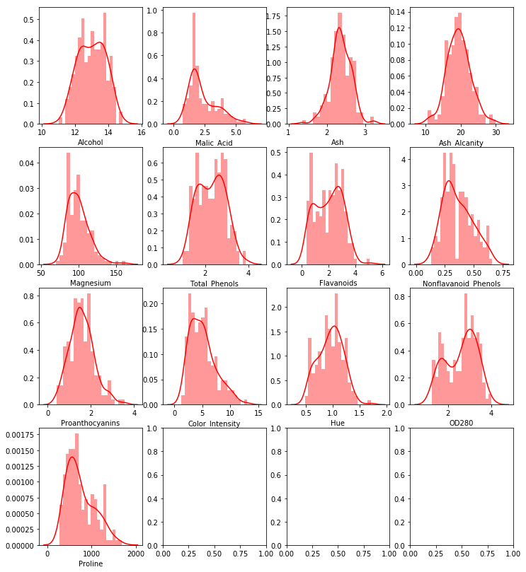
3.Data Analysis
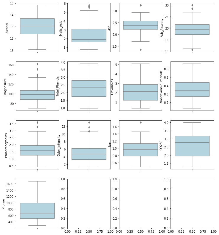
Skewness and Outliers and Correlation
def plot_multi_variable(row,column) :
    """
    Plot multi variables histogram for dataframe with row = row and colunm = column
    """
    _,ax = plt.subplots(row,column,figsize = (12,14))
    for i in range(0,row) :
        for j in range(0,column) :
            if (row*i + j >= df.shape[1]) :
                break
            else :
                sns.distplot(df.iloc[:,row*i+j],color = "red",bins = 20,ax = ax[i,j])

plot_multi_variable(4,4)
def plot_boxplot_multi_variable(row,column) :
    """
    Plot multi variables boxplot for dataframe with row = row and colunm = column
    """
    _,ax = plt.subplots(row,column,figsize = (12,14))
    for i in range(0,row) :
        for j in range(0,column) :
            if (row*i + j >= df.shape[1]) :
                break
            else :
                sns.boxplot(y = df.iloc[:,row*i+j],color = "lightblue",ax = ax[i,j])

plot_boxplot_multi_variable(4,4)
_,_= plt.subplots(1,1,figsize = (10,10))
corr = df.corr()
mask = np.zeros_like(corr)
mask[np.triu_indices_from(mask)] = True
sns.heatmap(corr,mask = mask,cmap=plt.cm.PuOr,square = True,annot = True)
<matplotlib.axes_subplots.AxesSubplot at 0x7f8ce7eddbe0>
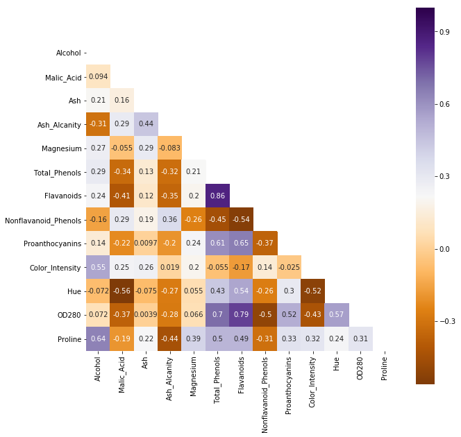
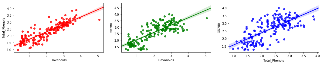
Flavanoids vs Total_Phenols : 0.86
OD280 vs Flavanoids : 0.79
OD280 vs Total_Phenols : 0.70
To large prob, these 3 variables are not I.I.D
_,ax = plt.subplots(1,3,figsize = (18,3))
sns.regplot(df["Flavanoids"],df["Total_Phenols"],ax = ax[0],color = "red")
sns.regplot(df["Flavanoids"],df["OD280"],ax = ax[1],color = "green")
sns.regplot(df["Total_Phenols"],df["OD280"],ax = ax[2],color = "blue")
<matplotlib.axes_subplots.AxesSubplot at 0x7f8cebdcb048>
4.Clustering
Kmeans is sensitive to Outliers and skewness.
Try to scale first
from sklearn.preprocessing import StandardScaler
from sklearn.pipeline import Pipeline
from sklearn.cluster import KMeans

pl = Pipeline([
    ("scale",StandardScaler()),
    ("Kmeans", KMeans(n_clusters = 2,random_state = 13))
])

kmeans = pl.fit(df)
# centroids
print(kmeans.steps[1][1].cluster_centers_)
# withinss, Total within-cluster sum of squares , larger the better
print(kmeans.steps[1][1].inertia_)
[[-0.31148001  0.33837268 -0.0499309   0.46976489 -0.3074597  -0.75037054
  -0.789532    0.56770273 -0.61153123  0.0982258  -0.5400717  -0.68516469
  -0.58021779]
 [ 0.32580094 -0.35393004  0.05222657 -0.49136328  0.32159578  0.78487033
   0.82583232 -0.59380401  0.63964761 -0.10274193  0.56490258  0.71666652
   0.60689447]]
1658.7588524290954
# decide how many clusters is better
withinss = []
for i in range(1,10) :
    pl = Pipeline([
    ("scale",StandardScaler()),
    ("Kmeans", KMeans(n_clusters = i,random_state = 13))
    ])
    kmeans = pl.fit(df)
    withinss.append(kmeans.steps[1][1].inertia_)
plt.plot(withinss)
plt.ylabel("Total within-cluster sum of squares")
plt.xlabel("Number of Cluster")
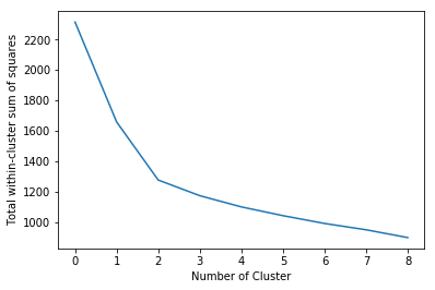
K = 3 is the optimized solution based on elbow criterion
When k = 3, cluster-inside sse is 1277 < 1658 when k = 2
pl_opt = Pipeline([
    ("scale",StandardScaler()),
    ("Kmeans", KMeans(n_clusters = 3,random_state = 13))
])

kmeans_opt = pl_opt.fit(df)
print(kmeans_opt.steps[1][1].inertia_)
1277.9284888446423
df["Cluster"] = kmeans_opt.steps[1][1].labels_
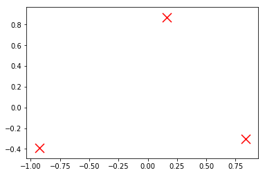
# Centroids
centroids = kmeans_opt.steps[1][1].cluster_centers_
plt.scatter(centroids[:, 0], centroids[:, 1],
            marker='x', s=169, linewidths=3,
            color='r', zorder=10)
<matplotlib.collections.PathCollection at 0x7f8cd9e50f60>
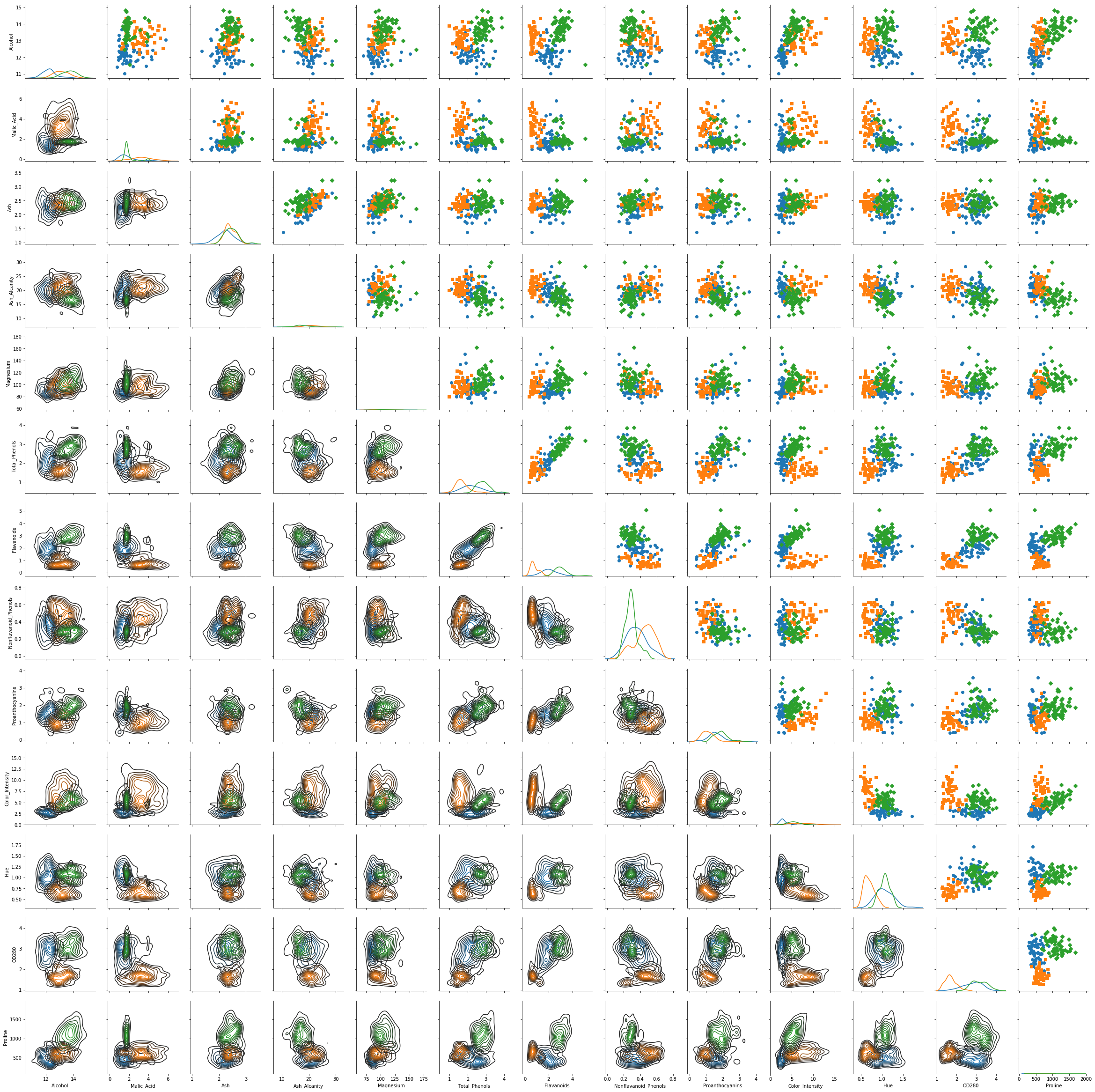
g = sns.PairGrid(df,hue = "Cluster",hue_kws={"marker": ["o", "s", "D"]},vars = df.columns[:df.shape[1]-1])
g = g.map_diag(sns.kdeplot)
g = g.map_upper(plt.scatter)
g = g.map_lower(sns.kdeplot)
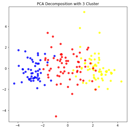
PCA analysis
from sklearn.decomposition import PCA
pipeline_pca = Pipeline([
    ("scale" , StandardScaler()),
    ("PCA" ,PCA(n_components = 13,random_state = 13))
])
pca_opt = pipeline_pca.fit_transform(df.drop("Cluster",axis = 1))
color = ["red" if i == 0 else "blue" if i == 1  else "yellow" for i in df["Cluster"]]
plt.figure(figsize = (7,7))
plt.scatter(pca_opt[:,0],pca_opt[:,2], c= color, alpha=0.8)
plt.title("PCA Decomposition with 3 Cluster")
plt.show()
5.Error Check
from sklearn.metrics import classification_report
label_new = ["A" if i == 1 else "B" if i == 2 else "C" for i in label]
Cluster_new = ["A" if i == 2 else "B" if i == 0 else "C" for i in df["Cluster"]]
print(classification_report(Cluster_new,label_new))
              precision    recall  f1-score   support

           A       1.00      0.95      0.98        62
           B       0.92      1.00      0.96        65
           C       1.00      0.94      0.97        51

   micro avg       0.97      0.97      0.97       178
   macro avg       0.97      0.96      0.97       178
weighted avg       0.97      0.97      0.97       178
# Accuracy
Correct = [1 if label_new[i] == Cluster_new[i] else 0 for i in range(0,len(label_new))]
print("Total Accuracy is :",np.mean(Correct))
Total Accuracy is : 0.9662921348314607