1. About This Database
I will use random generated data with same variables with the data in customer database since these customers data is confidential. Also I will use my own data as demo customer data to show how to get the estimated level for different variables.
There are some type of customer data : basic information; consumption attributes; habit attributes; wealthy attributes; location attributes and others :
Basic Information : Customer_Id, Name, Gender, Age, Education Level,Family Size
Consumption Attributes : Comsuption Frequency, Reason of Treatment, Payment Method, Credit
Habit Attributes : Treatment Duration, Treatment Type, Treatment Type
Wealth Attributes : Has Insurance, Insurance Company, Occupation, Estimated Salary
Location Attributes : Location Area
Advertising Attributes : How to know us, comment
Here is my own info and I will show how to do data cleaning and data preprocessing.
# import packages
import pandas as pd
import numpy as np
from sklearn.neighbors import KNeighborsClassifier
from scipy.cluster.hierarchy import dendrogram, linkage
import matplotlib.pyplot as plt
import seaborn as sns
from kmodes.kmodes import KModes
import gc
temp = pd.DataFrame(np.random.randint(0,11,size = (1,19)),
                    columns = list(["Customer_Id","Name","Gender","Age","EducationLevel","Occupation","FamilySize",
                                    "Comsumption_Freq","TreatmentReason","PaymentMethod","Credit","TreatmentDuration(mins)",
                                    "TreatmentType", "HasInsurance","InsuranceCompany","Income","Location","How_to_know_us",
                                    "Comment"]))
temp.loc[0,:] = [1,"Boyu_HA","male",28,"bachelor","analytics",3,"often","painful","debit card",
                 10,60,"RMT","yes","GreatWest Life","","1350 Birchmount RdScarborough, ON M1P 2E3",
                 "doctor referral",5]
temp
| Customer_Id | Name | Gender | Age | EducationLevel | Occupation | FamilySize | Comsumption_Freq | TreatmentReason | PaymentMethod | Credit | TreatmentDuration(mins) | TreatmentType | HasInsurance | InsuranceCompany | Income | Location | How_to_know_us | Comment | |
|---|---|---|---|---|---|---|---|---|---|---|---|---|---|---|---|---|---|---|---|
| 0 | 1 | Boyu_HA | male | 28 | bachelor | analytics | 3 | often | painful | debit card | 10 | 60 | RMT | yes | GreatWest Life | 1350 Birchmount RdScarborough, ON M1P 2E3 | doctor referral | 5 |
2. Data Cleaning
There are 17 variables in this dataframe, some of them are numeric variables while others are categorical. So I can’t use simple KMeans or Hierarchical Clustering since they are not available for two-type data.
One method to handle this is using One-Hot-Encoding, convert all categorical to numerical variables. Pros are : Simple to do, numeric data provides better clustering. Cons are : lost the relationship of categorical data.
Another method is just converting the numeric variables into categorical variables with range-gap, like Age 0-18 named as Teenager, Age 19 - 29 as Youth, Age 30 - 50 as Adult, Age larger than 50 as Senior and then convert these labels into numbers 1-4.
Third method is that we don’t convert any type but using orginal data directly with K-prototypes algorithm. (Here is the package description : https://github.com/nicodv/kmodes)
# copy database
df = temp.copy()
Age Group :
Group 1 : less than 18      ---- Teeneger
Group 2 : 18 - 29           ---- Youth
Group 3 : 30 - 49           ---- Adult
Group 4 : larger than 50    ---- Senior
# Convert Age into age-group
age_group = [1 if i < 18 else
             2 if i >18 & i<29 else
             3 if i >29 & i < 50 else
             4
             for i in df.Age]
df["age_group"] = age_group
gc.collect()
11076
Gender Group :
Group 0 : female
Group 1 : male
Group 2 : Others
# Convert gender into 0/1/2 : male 1 female 0 unknown 2
gender = [0 if i == "female" else
          1 if i == "male" else
          2
          for i in df.Gender]
df["Gender"] = gender
gc.collect()
0
Education Level :
Group 0 : High School
Group 1 : College
Group 2 : Bachelor Degree
Group 3 : Master Degree
Group 4 : Doctor Degree
Group 5 : Others
# Convert education level into number : high school : 0 college : 1 bachelor : 2 Master : 3 Doctor : 4
education = [0 if i == "high school" else
             1 if i == "college" else
             2 if i == "bachelor" else
             3 if i == "master" else
             4 if i == "doctor" else
             5
             for i in df.EducationLevel]
df["EducationLevel"] = education
gc.collect()
0
Occupation Group :
Based on government MOG-level (https://www.bls.gov/ncs/ocs/ocsm/comMOGADEF.htm), cluster different occupation into 11 groups, rating from A - K. I just convert them to 1 - 11.
# cluster occupation
df["Occupation"] = 1
Comsumption_Freq Group :
Group 0 : Never come before
Group 1 : Rare
Group 2 : Regualr
Group 3 : High Frequency
# Comsumption_Freq
Comsumption_Freq = [0 if i == "never" else
                    1 if i == "rare" else
                    2 if i == "regular" else
                    3
                    for i in df.Comsumption_Freq]
df["Comsumption_Freq"] = Comsumption_Freq
gc.collect()
0
Treatment Reason Group :
There are 3 main reason group : relax, painful, rehab
Group 0 : Relax
Group 1 : Painful
Group 2 : rehab
# There are two main parts of TreatmentReason : Relax : 0 and Painful : 1
TreatmentReason = [0 if i == "relax" else
                   1 if i == "painful" else
                   2
                   for i in df.TreatmentReason]
df["TreatmentReason"] = TreatmentReason
gc.collect()
0
Payment Method :
There are a few payment methods available :
Group 1 : Debit Card
Group 2 : Visa/Master
Group 3 : Insurance Visa
Group 4 : Check
Group 5 : Cash
Group 6 : Direct Billing
Group 7 : Gift Card
# Payment method
Payment = [1 if i == "debit card" else
           2 if (i == "visa"| i == "master") else
           3 if i == "insurance visa" else
           4 if i == "check" else
           5 if i == "cash" else
           6 if i == "direct billing" else
           7 if i == "gift card" else
           8
           for i in df.PaymentMethod]

df["PaymentMethod"] = Payment
gc.collect()
0
Credit
Credit is the credit record based on if there were late appointment or missed appointment or other payment problems rating from 0-10, 10 is the best
Treatment Type Group :
We have several treatment availables : RMT, Accupuncture, Osteopath, Physiotherapy and other treatments
Group 0 : RMT
Group 1 : Accupuncture
Group 2 : Osteopath
Group 3 : Physiotherapy
Group 4 : Others
TreatmentType = [0 if i == "RMT" else
                 1 if i == "Accupuncture" else
                 2 if i == "Osteopath" else
                 3 if i == "Physiotherapy" else
                 4
                 for i in df.TreatmentType]
df["TreatmentType"] = TreatmentType
gc.collect()
0
Has Insurance
logistic variables : Yes or No
Group 0 : No
Group 1 : Yes
# Has Insurance
HasInsurance = [0 if i == "no" else 1 for i in df.HasInsurance]
df["HasInsurance"] = HasInsurance
gc.collect()
0
Insurance Company
Based on Canadian Insurance Company List
0 : None
1 : Blue Cross
2 : Desjardins Group
3 : Empire Life
4 : Green Shield Canada
5 : The Great-West Life Assurance Company
6 : Manulife Financial
7 : Sun Life Financial
8 : TD Insurance
9 : Others
# InsuranceCompany
InsuranceCompany = [0 if i == "none" else
                    1 if i == "Blue Cross" else
                    2 if i == "Desjardins" else
                    3 if i == "Empire Life" else
                    4 if i == "Green Shield" else
                    5 if i == "Great-West Life" else
                    6 if i == "Manulife" else
                    7 if i == "Sun Life" else
                    8 if i == "TD Insurance" else
                    9
                    for i in df.InsuranceCompany]


df["InsuranceCompany"] = InsuranceCompany
gc.collect()
0
Income
There are some of information that nobody wants to get out, like marriage, income and other personal information. But they are one of key features for customer segmentation.
My soltuion to this is to estimate salary / income based on occupation estimated salary and working year.
For occupation estimated salary, code can be grabbed from my another project Indeed Analytics(https://tabrishaby.github.io/2018/02/15/Indeed-Data-Job-Python/)
Working year can be calculated by [Age - 22], 22 is the average college/university students graduation age.
company size coefficient : range from [0.5,1], the larger the number , the larger the company size
working year coefficient : range from [0.5,1], the larger the number , the longer the working years
estimated income = [occupation estimated salary] $\cdot$ [company size coefficient] $\cdot$ [working year coefficient]
Pros : Easy to access the data, methods make sense in some way.
Cons : Influence of unrelated working years, company size hard to estimate
Convert Salary to salary range :
Group 1 : < 24000
Group 2 : 24000 - 48000
Group 3 : 48000 - 72000
Group 4 : 72000 - 100000
Group 5 : > 100000
# income
df["Income_Range"] = 2
Location
Estimated distance from address to us by Python Google Map Distance Matrix
(https://github.com/googlemaps/google-maps-services-python/tree/master/googlemaps)
Then convert to distance range :
Group 1 : less than 1000m      : Walk-in Distance
Group 2 : 1000 - 5000m         : Near
Group 3 : 5000 - 300000m       : Driving Distance
Group 4 : 300000 - 500000m     : Far
Group 5 : greater than 500000m : City Distance
import googlemaps

gmaps = googlemaps.Client(key='API Key')

distance_m = gmaps.distance_matrix(df.Location,"884 Eglinton Ave. West,Toronto, ON M6C 2B6")

df["distance"] = distance_m["rows"][0]["elements"][0]["distance"]["value"]

print(distance_m)
print("-"*40)
print("Distance is {}".format(df.distance))
{'destination_addresses': ['884 Eglinton Ave W, Toronto, ON M6C 2B6, Canada'], 'origin_addresses': ['1350 Birchmount Rd, Scarborough, ON M1P 2E4, Canada'], 'rows': [{'elements': [{'distance': {'text': '21.6 km', 'value': 21570}, 'duration': {'text': '23 mins', 'value': 1396}, 'status': 'OK'}]}], 'status': 'OK'}
----------------------------------------
Distance is 0    21570
Name: distance, dtype: int64
# distance group
distance_group = [1 if i < 1000 else
                  2 if (i > 1000 & i < 5000) else
                  3 if (i > 5000 & i < 30000) else
                  4 if (i > 30000 & i < 500000) else
                  5
                  for i in df.distance]

df["distance"] = distance_group
gc.collect()
34
How to know us :
Advertising Attribues :
We have several advertising methods :
Insurance Referral, Doctor Referral, Google advertising, Apple/Bing Map, Magazine Advertising, Flyer

Group 1 : Insurance Referral
Group 2 : Doctor Referral
Group 3 : Google Advertising
Group 4 : Map
Group 5 : Magazine Advertising
Group 6 : Flyer
Group 7 : Others
# advertising group
how_to_know_us = [1 if i == "insurance referral" else
                  2 if i == "doctor referral" else
                  3 if i == "google advertising" else
                  4 if i == "map" else
                  5 if i == "magazine advertising" else
                  6 if i == "flyer" else
                  7
                  for i in df.How_to_know_us]

df.How_to_know_us = how_to_know_us
gc.collect()
0
Comment
Pickup review score only; ranking from 1-10
3. Data Preprocessing
I have already cleaned up the whole database, next step is to do the data preprocessing :
1. Convert Numeric to Categorical
2. Drop unrelated variables
3. Add some features.
4. Convert int64 to int8 to save spaces
# glimpse databse df
print(df.columns)
print("-"*40)
print(df.info())
print("-"*40)
print(df.head())
Index(['Customer_Id', 'Name', 'Gender', 'Age', 'EducationLevel', 'Occupation',
       'FamilySize', 'Comsumption_Freq', 'TreatmentReason', 'PaymentMethod',
       'Credit', 'TreatmentDuration(mins)', 'TreatmentType', 'HasInsurance',
       'InsuranceCompany', 'Income', 'Location', 'How_to_know_us', 'Comment',
       'age_group', 'Income_Range', 'distance'],
      dtype='object')
----------------------------------------
<class 'pandas.core.frame.DataFrame'>
RangeIndex: 1 entries, 0 to 0
Data columns (total 22 columns):
Customer_Id                1 non-null int32
Name                       1 non-null object
Gender                     1 non-null int64
Age                        1 non-null int32
EducationLevel             1 non-null int64
Occupation                 1 non-null int64
FamilySize                 1 non-null int32
Comsumption_Freq           1 non-null int64
TreatmentReason            1 non-null int64
PaymentMethod              1 non-null int64
Credit                     1 non-null int32
TreatmentDuration(mins)    1 non-null int32
TreatmentType              1 non-null int64
HasInsurance               1 non-null int64
InsuranceCompany           1 non-null int64
Income                     1 non-null object
Location                   1 non-null object
How_to_know_us             1 non-null int64
Comment                    1 non-null int32
age_group                  1 non-null int64
Income_Range               1 non-null int64
distance                   1 non-null int64
dtypes: int32(6), int64(13), object(3)
memory usage: 232.0+ bytes
None
----------------------------------------
   Customer_Id     Name  Gender  Age  EducationLevel  Occupation  FamilySize  \
0            1  Boyu_HA       1   28               2           1           3

   Comsumption_Freq  TreatmentReason  PaymentMethod    ...     TreatmentType  \
0                 3                1              1    ...                 0

   HasInsurance  InsuranceCompany  Income  \
0             1                 9

                                    Location How_to_know_us Comment  \
0  1350 Birchmount RdScarborough, ON M1P 2E3              2       5

   age_group  Income_Range  distance
0          2             2         2

[1 rows x 22 columns]
Drop columns :
Drop Name, Income, Location since already have better replacement.
# Drop columns
df = df.drop(["Name","Income","Location"],axis = 1)
Add Variables :
Add some variables that maybe related to result.
Insurance Type : Data collected from Insurance company, like health insurance, accident insurance, disability
                 insurance and so on.

Insurance Amount : Data collected from Insurance company. The total amount for customer/family, like $500,$1000

And So On.
There are some more info from insurance company I didn’t list.
# Add new columns

# Insurance Type
df["InsuraneType"] = 1

# Insurance Amount
df["InsuranceAmount"] = 2

# drop Age
df = df.drop(["Age"],axis = 1)
Data Conversion
Convert numeric data into categorical data
df = df.apply(lambda x : x.astype("category"))
4. Modeling
- Split data
- Principal Feature Analysis to check the importance of different features
- Modeling with different algorithms
- Visualization
# I will generate 1000 data record instead of my own data to show algorithms
data = pd.DataFrame(np.random.randint(0,11,size = (1000,12)),
                    columns = list(["Comsumption_Freq","","PaymentMethod","Credit","TreatmentDuration(mins)","Occupation"
                                    "InsuranceCompany","","InsuranceAmount","How_to_know_us","distance","","Location"]))

data["Gender"] = np.random.randint(0,2,size = (1000,1))
data["EducationLevel"] = np.random.randint(0,6,size = (1000,1))
data["age_group"] = np.random.randint(0,6,size = (1000,1))
data["FamilySize"] = np.random.randint(0,6,size = (1000,1))
data["TreatmentReason"] = np.random.randint(0,6,size = (1000,1))
data["TreatmentType"] = np.random.randint(0,6,size = (1000,1))
data["InsuraneType"] = np.random.randint(0,6,size = (1000,1))
data["Income_Range"] = np.random.randint(0,6,size = (1000,1))
data["Comment"] = np.random.randint(0,6,size = (1000,1))
data["HasInsurance"] = np.random.randint(0,2,size = (1000,1))


data = data.apply(lambda x : x.astype("category"))
# customer ID
Id = pd.Series(np.arange(1,1001))
Feature Importance
Consider if using feature importance selection, get the non-selection PCA result first
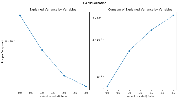
The Cumsum Variance is not so good at all since this is the randomly generated data. The real dataset has a far better result (90.2%).
# PCA

from sklearn.decomposition import PCA

pca_data = PCA(n_components=4).fit(data)

plt.subplots(figsize = (12,6))
plt.subplot(121)
plt.semilogy(pca_data.explained_variance_ratio_, '--o')
plt.xlabel("variables(sorted) Ratio")
plt.ylabel("Priciple Component")
plt.title("Explained Variance by Variables")

plt.subplot(122)
plt.semilogy(pca_data.explained_variance_ratio_.cumsum(), '--o')
plt.xlabel("variables(sorted) Ratio")
plt.title("Cumsum of Explained Variance by Variables")

plt.suptitle("PCA Visualization")

plt.show()

Feature Selection :
Select Top 10 features based on Variance.
# function of PFA
from sklearn.decomposition import PCA
from sklearn.cluster import KMeans
from collections import defaultdict
from sklearn.metrics.pairwise import euclidean_distances
from sklearn.preprocessing import StandardScaler

class PFA(object):
    def __init__(self, n_features, q=None):
        self.q = q
        self.n_features = n_features

    def fit(self, X):
        if not self.q:
            self.q = X.shape[1]

        sc = StandardScaler()
        X = sc.fit_transform(X)

        pca = PCA(n_components=self.q).fit(X)
        A_q = pca.components_.T

        kmeans = KMeans(n_clusters=self.n_features).fit(A_q)
        clusters = kmeans.predict(A_q)
        cluster_centers = kmeans.cluster_centers_

        dists = defaultdict(list)
        for i, c in enumerate(clusters):
            dist = euclidean_distances([A_q[i, :]], [cluster_centers[c, :]])[0][0]
            dists[c].append((i, dist))

        self.indices_ = [sorted(f, key=lambda x: x[1])[0][0] for f in dists.values()]
        self.features_ = X[:, self.indices_]
pfa = PFA(n_features = 10)
pfa.fit(data)

# To get the transformed matrix
X = pfa.features_

# To get the column indices of the kept features
column_indices = pfa.indices_
# assign top 10 features to selected_data
selected_data = data[data.columns[column_indices]]
Hierarchy
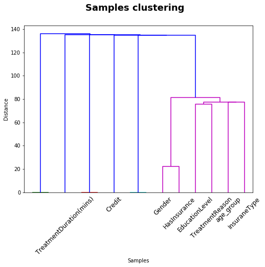
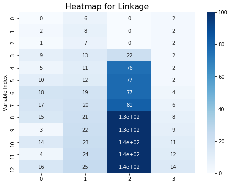
Visualize hierarchy of different variables
from scipy.spatial.distance import pdist, squareform
from scipy.cluster.hierarchy import linkage, dendrogram
data_dist = pdist(selected_data.T) # computing the distance
data_link = linkage(selected_data.T) # computing the linkage
# plot dendrogram of top variance explained variables
fig = plt.figure(figsize = (8,6))

dendrogram(data_link,labels=selected_data.columns)
plt.xticks(rotation = 45)
plt.xlabel('Samples')
plt.ylabel('Distance')
plt.suptitle('Samples clustering', fontweight='bold', fontsize=18)
plt.show()

plt.figure(figsize = (8,6))
sns.heatmap(data_link,annot = True,vmin = 0,vmax = 100,cmap = "Blues")
plt.title("Heatmap for Linkage",fontsize = 16)
plt.ylabel("Variable Index")

plt.show()

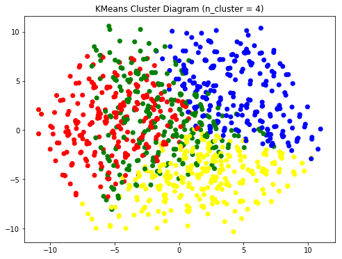
Kmeans Diagram
# kmeans cluster
km = KMeans(n_clusters = 4)

# predict the cluster
Cluster = km.fit(selected_data).labels_
# PCA to reduce dimension to 2 -D
pca_red = PCA(n_components = 2)
pca_red_fit = pca_red.fit_transform(selected_data)
x = pca_red_fit[:,0]
y = pca_red_fit[:,1]

# set up plotting dataframe
plot_df = pd.DataFrame({"CustomerID" : Id,
                        "Cluster" : Cluster,
                        "X" : x,
                        "Y" : y})
# color list
c = ["red" if i == 0 else
     "green" if i == 1 else
     "yellow" if i == 2 else
     "blue"
     for i in plot_df.Cluster]

# scatter plot
plt.figure(figsize = (8,6))
plt.scatter(x = plot_df["X"],y = plot_df["Y"], c = c)
plt.title("KMeans Cluster Diagram (n_cluster = 4)")
plt.show()

Conclusion
We can do further study based on the result we have now.
Study the detail attributes for different cluster, figure out the importance of each variable for future database improvement.

Label each cluster and apply different strategies :

        - For Non-regular and Protential customers, provide them some promotion and/or packages to attract them.
        For this cluster clients, price rate is already more important.

        - For Impossible customers, provide them blog articles and scientific survey paper on the importance of
        treatments on their health. When they start to be interested in these info, listing them to protential
        customer and apply the strategy above. Another possible method is that, based on my survey, more than
        40% of people who has insurance but never use them, I can let them know that they will lose money if they
        don't use up them.

        - For loyalty customers, however, I suggest that to satisfy them mentally is more important than the price
        or treatment itself. Regular customers, to a large extent, means they already satisfy with treatment,rate,
        environment and are happy with the therapies, so a sense of belonging is more important for them. We can
        send them mails or a little gift on their birthday and Chirstmas or New Year Day and so on.

Check up the effect of different adverstising, increase funding for the useful one.