Part I : Analysis Preparation
# import packages

# basic packages
import pandas as pd
import matplotlib.pyplot as plt
import seaborn as sns
import numpy as np
import random

# general packages
import warnings
warnings.filterwarnings('ignore')
%matplotlib inline

# model packages
from sklearn import linear_model
from sklearn.linear_model import ElasticNet, Lasso,  Ridge, LassoLarsIC, LinearRegression, LogisticRegression
from sklearn.ensemble import RandomForestRegressor,  GradientBoostingRegressor
from sklearn.metrics import mean_squared_error
import xgboost
from sklearn.model_selection import train_test_split

# Model Tune packages
from sklearn.model_selection import GridSearchCV

# CV Folder
from sklearn.model_selection import cross_validate
from sklearn.model_selection import cross_val_score
from sklearn.model_selection import ShuffleSplit
# load train/test data
train = pd.read_csv('../input/train.csv')
test = pd.read_csv('../input/test.csv')
df = pd.concat((train, test)).reset_index(drop=True)

# basic info
print('Shape of Train: ',train.shape)
print('-'*40)
print('Shape of Test: ',test.shape)
print('-'*40)
print(train.columns)
print('-'*40)
print(test.columns)
Shape of Train:  (1460, 81)
----------------------------------------
Shape of Test:  (1459, 80)
----------------------------------------
Index(['Id', 'MSSubClass', 'MSZoning', 'LotFrontage', 'LotArea', 'Street',
       'Alley', 'LotShape', 'LandContour', 'Utilities', 'LotConfig',
       'LandSlope', 'Neighborhood', 'Condition1', 'Condition2', 'BldgType',
       'HouseStyle', 'OverallQual', 'OverallCond', 'YearBuilt', 'YearRemodAdd',
       'RoofStyle', 'RoofMatl', 'Exterior1st', 'Exterior2nd', 'MasVnrType',
       'MasVnrArea', 'ExterQual', 'ExterCond', 'Foundation', 'BsmtQual',
       'BsmtCond', 'BsmtExposure', 'BsmtFinType1', 'BsmtFinSF1',
       'BsmtFinType2', 'BsmtFinSF2', 'BsmtUnfSF', 'TotalBsmtSF', 'Heating',
       'HeatingQC', 'CentralAir', 'Electrical', '1stFlrSF', '2ndFlrSF',
       'LowQualFinSF', 'GrLivArea', 'BsmtFullBath', 'BsmtHalfBath', 'FullBath',
       'HalfBath', 'BedroomAbvGr', 'KitchenAbvGr', 'KitchenQual',
       'TotRmsAbvGrd', 'Functional', 'Fireplaces', 'FireplaceQu', 'GarageType',
       'GarageYrBlt', 'GarageFinish', 'GarageCars', 'GarageArea', 'GarageQual',
       'GarageCond', 'PavedDrive', 'WoodDeckSF', 'OpenPorchSF',
       'EnclosedPorch', '3SsnPorch', 'ScreenPorch', 'PoolArea', 'PoolQC',
       'Fence', 'MiscFeature', 'MiscVal', 'MoSold', 'YrSold', 'SaleType',
       'SaleCondition', 'SalePrice'],
      dtype='object')
----------------------------------------
Index(['Id', 'MSSubClass', 'MSZoning', 'LotFrontage', 'LotArea', 'Street',
       'Alley', 'LotShape', 'LandContour', 'Utilities', 'LotConfig',
       'LandSlope', 'Neighborhood', 'Condition1', 'Condition2', 'BldgType',
       'HouseStyle', 'OverallQual', 'OverallCond', 'YearBuilt', 'YearRemodAdd',
       'RoofStyle', 'RoofMatl', 'Exterior1st', 'Exterior2nd', 'MasVnrType',
       'MasVnrArea', 'ExterQual', 'ExterCond', 'Foundation', 'BsmtQual',
       'BsmtCond', 'BsmtExposure', 'BsmtFinType1', 'BsmtFinSF1',
       'BsmtFinType2', 'BsmtFinSF2', 'BsmtUnfSF', 'TotalBsmtSF', 'Heating',
       'HeatingQC', 'CentralAir', 'Electrical', '1stFlrSF', '2ndFlrSF',
       'LowQualFinSF', 'GrLivArea', 'BsmtFullBath', 'BsmtHalfBath', 'FullBath',
       'HalfBath', 'BedroomAbvGr', 'KitchenAbvGr', 'KitchenQual',
       'TotRmsAbvGrd', 'Functional', 'Fireplaces', 'FireplaceQu', 'GarageType',
       'GarageYrBlt', 'GarageFinish', 'GarageCars', 'GarageArea', 'GarageQual',
       'GarageCond', 'PavedDrive', 'WoodDeckSF', 'OpenPorchSF',
       'EnclosedPorch', '3SsnPorch', 'ScreenPorch', 'PoolArea', 'PoolQC',
       'Fence', 'MiscFeature', 'MiscVal', 'MoSold', 'YrSold', 'SaleType',
       'SaleCondition'],
      dtype='object')
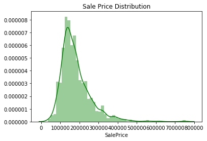
The traget is saleprice, so we analyze it first. it seems that the plot is not normal distribution since it has left skewness with large right tail. I will get skewness and kurtosis to comfirm this. If so, I will try to scale the data for further analysis.
# saleprice
g = sns.distplot(train.SalePrice,color = 'g')
g.set_title('Sale Price Distribution')
plt.show()
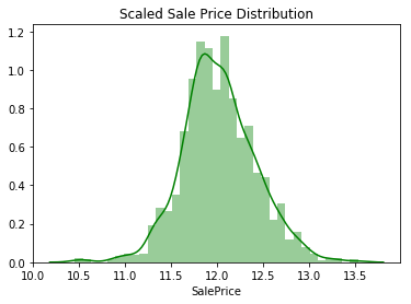
# scale sale price
df['SalePrice'] = np.log1p(df['SalePrice'])

# plot and cjeck
g1 = sns.distplot(df[:1460].SalePrice,color = 'g')
g1.set_title('Scaled Sale Price Distribution')

plt.show()
# skewness and kurtosis
print('Skewness is: ', train.SalePrice.skew())
print('-'*40)
print('Kurtosis is: ',train.SalePrice.kurt())
Skewness is:  1.88287575977
----------------------------------------
Kurtosis is:  6.53628186006
Part 2 : EDA
- General Visualization
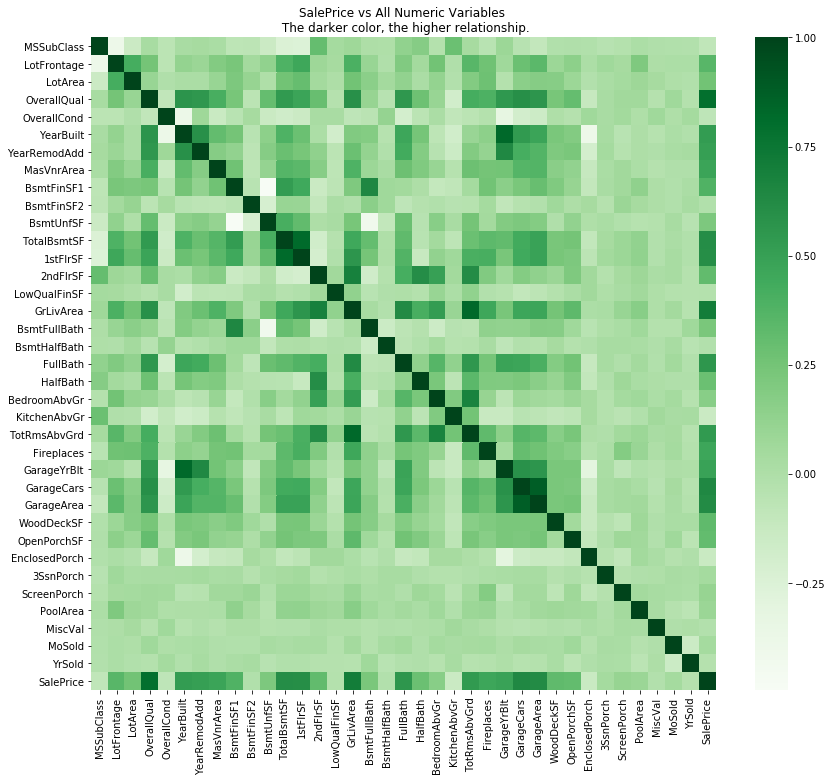
# Using Corraltion matrix to analyze numeric data first
_,ax = plt.subplots(figsize=(14,12))
sns.heatmap(train.drop('Id',axis = 1).corr(),cmap = 'Greens')
ax.set_title('SalePrice vs All Numeric Variables \n The darker color, the higher relationship.')
plt.show()
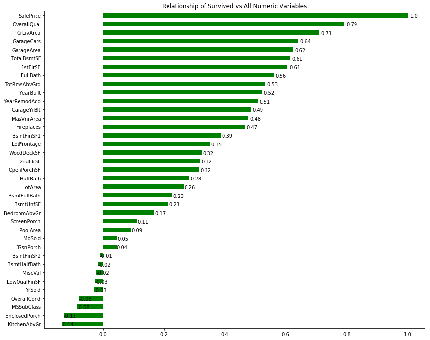
# list relationship of all numeric variables with SalePrice
_,ax = plt.subplots(figsize = (14,12))
g = train.drop(['Id'],axis = 1).corr()['SalePrice'].sort_values().plot.barh(color = 'g')
ax.set_title('Relationship of Survived vs All Numeric Variables')

# add annotation
for p in g.patches:
    g.annotate(str(round(p.get_width(),2)), (p.get_width() * 1.01,p.get_y()))

plt.show()
2.Imputation Missing Values
# plot all missing values
_,ax = plt.subplots(1,2,figsize = (14,8))
g1 = df.isnull().sum().sort_values(ascending = False).head(30).plot.barh(ax = ax[0],color = 'g')
g2 = train.isnull().sum().sort_values(ascending = False).head(20).plot.barh(ax = ax[1],color = 'g')
g1.set_title('Missing Values for All Data')
g2.set_title('Missing Values fro Train')

# add annotation
for p in g1.patches:
    g1.annotate(str(round(p.get_width(),2)), (p.get_width() * 1.01,p.get_y()))

plt.show()
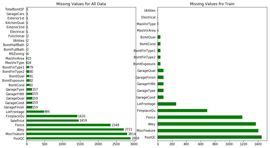
# drop columns with more than 600 missings values, eg ('PoolQC','MiscFeature','Alley','Fence','FireplaceQu')
df = df.drop(['PoolQC','MiscFeature','Alley','Fence','FireplaceQu'],axis = 1)
print(df.shape)
(2919, 76)
-
Fill na of LotFrontage with neighbourhood since houses in same neighbor should have same distince to road.
-
Garage group : there are 157 houses don’t have any info of garage, I’ m suppose that they dont have garage, while 2 of them have the garage type info, I will try to imputate them.
-
Basement group : 79 of them dont have any basement info, I’m supposed they dont have basement, and impute others.
-
MasVnr group : 23 of them fill na with None and imputate the last one.
-
Imputate other individuals
# LotFrontage : immutate with neighborhood variables
df['LotFrontage'] = df.groupby(['Neighborhood'])['LotFrontage'].transform(lambda x: x.fillna(x.median()))
for col in ('GarageType', 'GarageFinish', 'GarageQual', 'GarageCond'):
    df[col] = df[col].fillna('None')
for col in ('GarageYrBlt', 'GarageArea', 'GarageCars'):
    df[col] = df[col].fillna(0)
for col in ('BsmtFinSF1', 'BsmtFinSF2', 'BsmtUnfSF','TotalBsmtSF', 'BsmtFullBath', 'BsmtHalfBath'):
    df[col] = df[col].fillna(0)
for col in ('BsmtQual', 'BsmtCond', 'BsmtExposure', 'BsmtFinType1', 'BsmtFinType2'):
    df[col] = df[col].fillna('None')
df["MasVnrType"] = df["MasVnrType"].fillna("None")
df["MasVnrArea"] = df["MasVnrArea"].fillna(0)
# MSZoning
print(df['MSZoning'].describe()) # top is RL
df['MSZoning'] = df['MSZoning'].fillna('RL')
count     2915
unique       5
top         RL
freq      2265
Name: MSZoning, dtype: object
# Utilities
df['Utilities'].value_counts() # there are 2916 allpub and 1 Nosewa and 2 NAs, drop this variable
df = df.drop('Utilities',axis = 1)
# Functional
print(df['Functional'].value_counts()) # top is Typ
df['Functional'] = df['Functional'].fillna('Typ')
Typ     2717
Min2      70
Min1      65
Mod       35
Maj1      19
Maj2       9
Sev        2
Name: Functional, dtype: int64
# Exterior1st / Exterior2nd
print(df['Exterior1st'].value_counts()) # top is VinylSd and ImStucc only has 1 row, can be deleted when get_dummies
print(df['Exterior2nd'].value_counts()) # top is VinylSd and Other only has 1 row, can be deleted when get_dummies
df['Exterior1st'] = df['Exterior1st'].fillna('VinylSd')
df['Exterior2nd'] = df['Exterior2nd'].fillna('VinylSd')
VinylSd    1025
MetalSd     450
HdBoard     442
Wd Sdng     411
Plywood     221
CemntBd     126
BrkFace      87
WdShing      56
AsbShng      44
Stucco       43
BrkComm       6
Stone         2
AsphShn       2
CBlock        2
ImStucc       1
Name: Exterior1st, dtype: int64
VinylSd    1014
MetalSd     447
HdBoard     406
Wd Sdng     391
Plywood     270
CmentBd     126
Wd Shng      81
BrkFace      47
Stucco       47
AsbShng      38
Brk Cmn      22
ImStucc      15
Stone         6
AsphShn       4
CBlock        3
Other         1
Name: Exterior2nd, dtype: int64
# KitchenQual
print(df['KitchenQual'].value_counts())
df['KitchenQual'] = df['KitchenQual'].fillna('TA')
TA    1492
Gd    1151
Ex     205
Fa      70
Name: KitchenQual, dtype: int64
# SaleType
print(df['SaleType'].value_counts())
df['SaleType'] = df['SaleType'].fillna('WD')
WD       2525
New       239
COD        87
ConLD      26
CWD        12
ConLI       9
ConLw       8
Oth         7
Con         5
Name: SaleType, dtype: int64
# Electrical
print(df['Electrical'].value_counts()) # top is SBrkr and Mix has only 1 row, deletes when get_dummies
df['Electrical'] = df['Electrical'].fillna('SBrkr')
SBrkr    2671
FuseA     188
FuseF      50
FuseP       8
Mix         1
Name: Electrical, dtype: int64
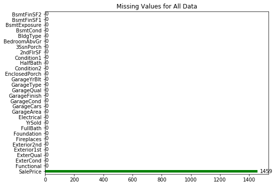
_,ax = plt.subplots(figsize = (8,6))
g1 = df.isnull().sum().sort_values(ascending = False).head(30).plot.barh(color = 'g')
g1.set_title('Missing Values for All Data')
for p in g1.patches:
    g1.annotate(str(round(p.get_width(),2)), (p.get_width() * 1.01,p.get_y()))
plt.show()
3.Outliers
_,ax = plt.subplots(3,2,figsize = (14,14))
sns.regplot(x = df.GrLivArea,y = df.SalePrice,ax = ax[0,0])
sns.regplot(x = df.TotalBsmtSF,y = df.SalePrice,ax = ax[0,1])
sns.boxplot(x = df.OverallCond,y = df.SalePrice,ax = ax[1,0])
sns.boxplot(x = df.OverallQual,y = df.SalePrice,ax = ax[1,1])
sns.regplot(x = df['1stFlrSF'],y = df.SalePrice,ax = ax[2,0])
sns.regplot(x = df['2ndFlrSF'],y = df.SalePrice, ax = ax[2,1])
<matplotlib.axes_subplots.AxesSubplot at 0x7fd57be72390>
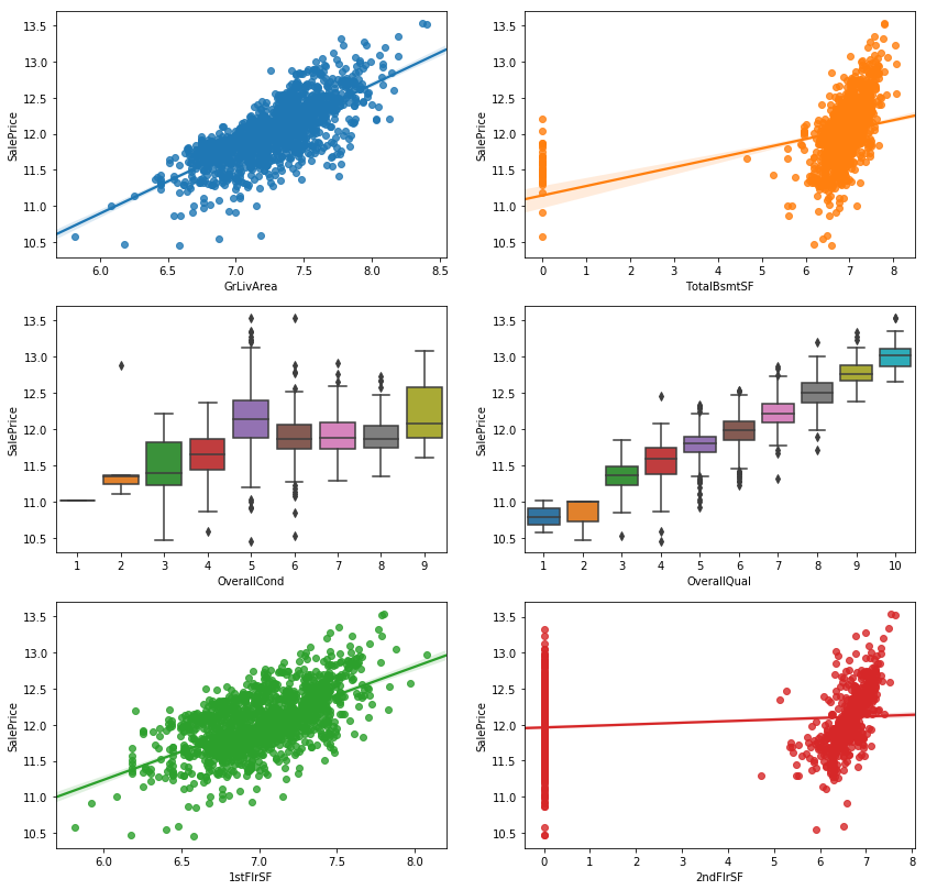
- Two Outliers in GrLivArea since they are too far away from fitted line.
- One outlier in TotalBsmtSF. If this house is the same one who is outlier in GrlivArea,then can be considerd as a really large house while in a bad location so the price is not so high as regular.
- One Outlier in OverallCond = 2 while it doesnt exist in OverallQual, means this house in low OverallCond butin a high OverallQual, which doesnt make sense based on the relationship of OverallCond and OverallQual, considered it as outlier.
- One Outlier in 1stFlrSF, i ‘m supposed to consider it as the same house. Delete it if so.
- For 2ndFlrSF, it doesn’t fit so well.
_,ax = plt.subplots(2,2,figsize = (14,10))
sns.boxplot(y = df.GarageArea,x = df.GarageCars,ax = ax[1,0])
sns.regplot(x = df['GarageArea'],y = df.SalePrice, ax = ax[0,1])
sns.boxplot(y = df.SalePrice,x = df.GarageCars,ax = ax[0,0])
sns.regplot(x = df['GarageArea']/df.GarageCars,y = df.SalePrice, ax = ax[1,1])

ax[0,0].set_title('GarageCars vs SalePrice')
ax[0,1].set_title('GarageAarea vs SalePrice')
ax[1,0].set_title('GarageCars vs GarageArea')
ax[1,1].set_title('GarageCars vs GarageArea Per Cars')
Text(0.5,1,'GarageCars vs GarageArea Per Cars')
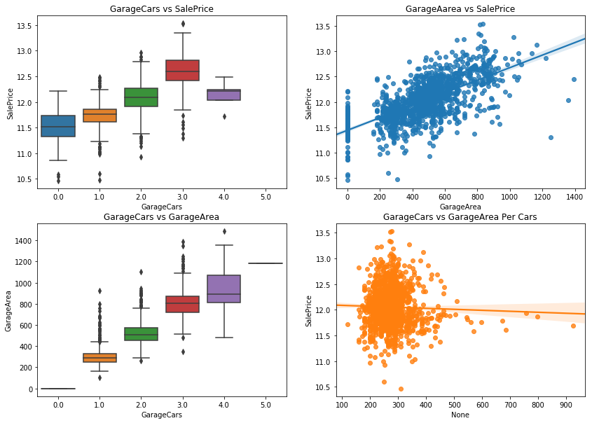
- Garage cars = 4, the saleprice suddenly dropped. And in test dataset there are some garagecars = 5 while there are none in train dataset.
- There are 4 extremely points in GarageArea plot.
- GarageArea and garagecars have strongly relationship with each other.
- Most of area for each cars are in 150 - 450 feets, while there are house with large area for each car
# drop outliers from GrLivArea and TotalBsmtSF plot
df = df.drop(df[df['Id'] == 1299].index)
df = df.drop(df[df['Id'] == 524].index)
# watch out there is one extremely point in test data too.
4.Scale data
scaled = ["1stFlrSF","2ndFlrSF","3SsnPorch","BsmtFinSF1","BsmtFinSF2","BsmtUnfSF","EnclosedPorch",
          "GarageArea","GrLivArea","LotArea","LotFrontage","LowQualFinSF","MasVnrArea","MiscVal",
          "OpenPorchSF","PoolArea","ScreenPorch","TotalBsmtSF", "WoodDeckSF"]
# ckech kurtosis and skewness
def skew_kur(df) :
    # select numeric variables
    num = []
    for c in df.columns :
        if c in scaled:
            num.append(c)
    # skewness
    skewness = []
    for c in num :
        skewness.append(df[c].skew())
    # kurtosis
    kurtosis = []
    for c in num :
        kurtosis.append(df[c].kurtosis())
    # norm dataframe
    norm = pd.DataFrame({'Variable' : num,
                        'skewness' : skewness,
                        'kurtosis' : kurtosis})
    return norm

norm = skew_kur(df)
skew_kur(df)
| Variable | kurtosis | skewness | |
|---|---|---|---|
| 0 | 1stFlrSF | 5.075293 | 1.257933 |
| 1 | 2ndFlrSF | -0.424185 | 0.861999 |
| 2 | 3SsnPorch | 149.304586 | 11.377932 |
| 3 | BsmtFinSF1 | 1.427134 | 0.981149 |
| 4 | BsmtFinSF2 | 18.828682 | 4.146636 |
| 5 | BsmtUnfSF | 0.403042 | 0.920161 |
| 6 | EnclosedPorch | 28.358039 | 4.004404 |
| 7 | GarageArea | 0.864865 | 0.216968 |
| 8 | GrLivArea | 2.456625 | 1.069300 |
| 9 | LotArea | 275.639934 | 13.116240 |
| 10 | LotFrontage | 8.526991 | 1.103332 |
| 11 | LowQualFinSF | 174.810242 | 12.090757 |
| 12 | MasVnrArea | 9.457156 | 2.623068 |
| 13 | MiscVal | 563.687542 | 21.950962 |
| 14 | OpenPorchSF | 11.021266 | 2.530660 |
| 15 | PoolArea | 327.027992 | 17.697766 |
| 16 | ScreenPorch | 17.761714 | 3.947131 |
| 17 | TotalBsmtSF | 3.711566 | 0.672097 |
| 18 | WoodDeckSF | 6.750566 | 1.845741 |
# consider -0.8 to 0.8 for skewness and -3.0 to 3.0 for kurtosis as the acceptable ranege to ensure 95% CI.
temp = norm[(abs(norm['kurtosis']) > 3) | (abs(norm['skewness']) > 0.8)]['Variable']

df[temp] = df[temp].apply(lambda x: np.log1p(x))
# double check
skew_kur(df)
# there are still some extremely value but much better
| Variable | kurtosis | skewness | |
|---|---|---|---|
| 0 | 1stFlrSF | 0.043907 | 0.030374 |
| 1 | 2ndFlrSF | -1.886414 | 0.306786 |
| 2 | 3SsnPorch | 76.527700 | 8.826656 |
| 3 | BsmtFinSF1 | -1.468428 | -0.616808 |
| 4 | BsmtFinSF2 | 4.248768 | 2.462526 |
| 5 | BsmtUnfSF | 3.953316 | -2.155250 |
| 6 | EnclosedPorch | 1.970906 | 1.960960 |
| 7 | GarageArea | 0.864865 | 0.216968 |
| 8 | GrLivArea | 0.103405 | -0.022062 |
| 9 | LotArea | 3.751081 | -0.532920 |
| 10 | LotFrontage | 2.744406 | -1.069416 |
| 11 | LowQualFinSF | 72.258633 | 8.559041 |
| 12 | MasVnrArea | -1.584435 | 0.538731 |
| 13 | MiscVal | 25.968860 | 5.214687 |
| 14 | OpenPorchSF | -1.773013 | -0.041559 |
| 15 | PoolArea | 243.656301 | 15.631314 |
| 16 | ScreenPorch | 6.755490 | 2.946085 |
| 17 | TotalBsmtSF | 25.569296 | -4.966774 |
| 18 | WoodDeckSF | -1.892872 | 0.159605 |
6.Add Features
- if house has Pool
- if house has garage
- Year/ month sold influence
- Neighborhood class
# HasPool : if poolarea != 0 then haspool = 1
df['HasPool'] = 0
df[df.PoolArea != 0]['HasPool'] = 1

# HasGarage : if garageyrblt =0 then hasgarage = 0
df['HasGarage'] = 0
df[df.GarageYrBlt != 0]['HasGarage'] = 1
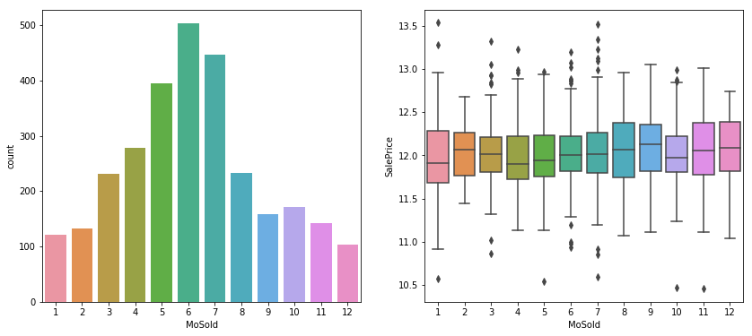
# Month
_,ax = plt.subplots(1,2,figsize = (14,6))
sns.countplot(df.MoSold,ax =ax[0])
sns.boxplot(x = df.MoSold,y = df.SalePrice,ax = ax[1])
<matplotlib.axes_subplots.AxesSubplot at 0x7fd5d5a92f60>
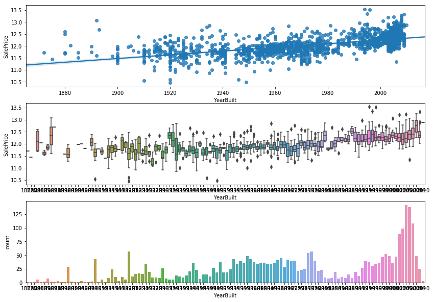
# Built year
_,ax = plt.subplots(3,1,figsize = (14,10))
sns.regplot(x = df.YearBuilt.astype(int),y = df.SalePrice,ax = ax[0])
sns.boxplot(x = df.YearBuilt.astype(int),y = df.SalePrice,ax =ax[1])
sns.countplot(df.YearBuilt.astype(int),ax =ax[2])
<matplotlib.axes_subplots.AxesSubplot at 0x7fd5d57f7d68>
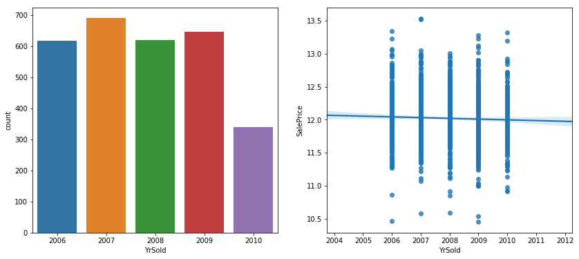
_,ax = plt.subplots(1,2,figsize = (14,6))
sns.countplot(df.YrSold,ax = ax[0])
sns.regplot(x = df.YrSold.astype(int),y = df.SalePrice,ax = ax[1] )
<matplotlib.axes_subplots.AxesSubplot at 0x7fd57ba0d128>
- In May, June and July, more houses sold, considered them as ‘HotMon’ while price is almost same
- The newer the houses, the more expensive they are.And more houses were built after 2000.
- The amount of houses sold in each houses were almost same while the trend of the saleprice descreased.
# Hot Mon
df['HotMon'] = 0
df[df.MoSold == 5|6|7]['HotMon'] =1

# HouseAge : YearSold - YearBuilt
df['HouseAge'] = df.YrSold.astype(int) - df.YearBuilt.astype(int)
# Neighborhood
_,ax = plt.subplots(2,1,figsize = (14,8))
sns.countplot(df.Neighborhood,ax = ax[0])
sns.boxplot(x = df.Neighborhood,y = df.SalePrice,ax = ax[1])
# consider average of each Neighborhood > 12.5 as 'ClassI' and others as 'Others'
print(df.groupby('Neighborhood')['SalePrice'].mean().sort_values(ascending = False).head())

# classI
df['ClassI'] = 0
df[(df.Neighborhood == 'NoRidge')|(df.Neighborhood =='NridgHt')|(df.Neighborhood =='StoneBr')]['ClassI'] = 1
Neighborhood
NoRidge    12.676003
NridgHt    12.619415
StoneBr    12.585490
Timber     12.363460
Veenker    12.344180
Name: SalePrice, dtype: float64
# TotalArea = basement + 1stfloor + 2ndfloor
df['TotalArea'] = df['1stFlrSF'] +df['2ndFlrSF'] +df['TotalBsmtSF']

# street tp 0/1
df.Street.replace(['Grvl', 'Pave'],[0,1],inplace = True)
7.Get Dummies
df_dummy = pd.get_dummies(df)
print(df_dummy.shape)
(2917, 283)
# drop some columns
# Exterior1st :ImStucc
# Exterior2nd :Other
# Electrical :Mix
df_dummy.drop(['Exterior1st_ImStucc','Exterior2nd_Other','Electrical_Mix'],axis = 1,inplace = True)
df_dummy.shape
(2917, 280)
# seperate train and test
train_dummy = df_dummy[:train.shape[0]-2] # 2 outliers
test_dummy = df_dummy[train.shape[0]-2:]
print(train_dummy.shape,test_dummy.shape)
(1458, 280) (1459, 280)
Part 3: Modeling
Level one model I want to use
 ----------------------------------------
   Linear
   LASSO
   Ridge
   Elastic Net
   Random Forest
   Gradient Boosting classifer
   XGBoost
 ----------------------------------------
# set up train/ test /traget / data dataset
train_Price = train_dummy['SalePrice'] # target
train_data = train_dummy.drop(['SalePrice','Id'],axis = 1) # data
print(train_Price.shape,train_data.shape)
(1458,) (1458, 278)
# train test split for scoring
x_train,x_test,y_train,y_test = train_test_split(train_data,train_Price,
                                               test_size = 0.25,random_state = 13)
print(x_train.info())
<class 'pandas.core.frame.DataFrame'>
Int64Index: 1093 entries, 669 to 338
Columns: 278 entries, 1stFlrSF to SaleType_WD
dtypes: float64(24), int64(19), uint8(235)
memory usage: 626.6 KB
None
# set up dataframe to see rmse
models = pd.DataFrame({
    'Model': ['Linear', 'Lasso', 'Ridge',
              'Elastic Net', 'Gradient Boosting', 'Random Forest',
              'Xgboost'],
    'Result': [ np.sqrt(mean_squared_error(LinearRegression().fit(x_train,y_train).predict(x_test),y_test)),
              np.sqrt(mean_squared_error(Lasso().fit(x_train,y_train).predict(x_test),y_test)),
              np.sqrt(mean_squared_error(Ridge().fit(x_train,y_train).predict(x_test),y_test)),
              np.sqrt(mean_squared_error(ElasticNet().fit(x_train,y_train).predict(x_test),y_test)),
              np.sqrt(mean_squared_error(GradientBoostingRegressor().fit(x_train,y_train).predict(x_test),y_test)),
              np.sqrt(mean_squared_error(RandomForestRegressor().fit(x_train,y_train).predict(x_test),y_test)),
              np.sqrt(mean_squared_error(xgboost.XGBRegressor().fit(x_train,y_train).predict(x_test),y_test))
              ]})
print(models.sort_values(by='Result'))
g = models.plot(kind = 'bar',title = 'Models RMSE Score \n The Lower the Better')
g.set_xlabel(list(models['Model']))
               Model    Result
2              Ridge  0.119638
0             Linear  0.125658
4  Gradient Boosting  0.136083
6            Xgboost  0.139107
5      Random Forest  0.164620
3        Elastic Net  0.253736
1              Lasso  0.258744


Text(0.5,0,"['Linear', 'Lasso', 'Ridge', 'Elastic Net', 'Gradient Boosting', 'Random Forest', 'Xgboost']")
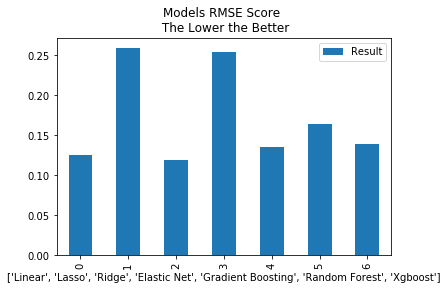
- RMSE is not so good as I think, consider CV folder with SearchGrid for better result.
- L2 regression is better than L1 regression
- Hyper Parameter Tuning for better results and ensemble models.
# split cv folder
cv_split = ShuffleSplit(n_splits = 10, test_size = .3,
                                        train_size = .6, random_state = 13)

# models will test
mod = [LinearRegression(),Lasso(),Ridge(),ElasticNet(),GradientBoostingRegressor(),RandomForestRegressor(),xgboost.XGBRegressor()]

# Cross validation
cv_score = list()
for model in mod :
    cv_result = np.sqrt(-cross_val_score(model, train_data, train_Price, cv  = cv_split,scoring='mean_squared_error'))
    cv_score.append(cv_result.mean())

cv_model = pd.DataFrame({
        'Model': ['Linear', 'Lasso', 'Ridge',
              'Elastic Net', 'Gradient Boosting', 'Random Forest',
              'Xgboost'],
        'CV Result' :cv_score})
print(cv_model.sort_values(by='CV Result'))
   CV Result              Model
2   0.119145              Ridge
0   0.129010             Linear
6   0.130008            Xgboost
4   0.130840  Gradient Boosting
5   0.153474      Random Forest
3   0.263963        Elastic Net
1   0.268069              Lasso
- Hyper parameters tunes
# Lasso
Lasso().get_params()
param_grid = {'alpha' : [0.0005,0.005,0.05,0.2,0.4],
              'tol': [0.1,0.01,0.001, 0.0001],
              'random_state' : [13]}
tuned_lasso = GridSearchCV(Lasso(),param_grid=param_grid, scoring = 'neg_mean_squared_error', cv = cv_split)
tuned_lasso.fit(train_data,train_Price)
print("Best Hyper Parameters:\n",tuned_lasso.best_params_)
Best Hyper Parameters:
 {'alpha': 0.0005, 'random_state': 13, 'tol': 0.01}
# Ridge
Ridge().get_params()
param_grid = {'alpha' : [0.005,0.05,0.2,0.4,0.6,1],
              'tol': [0.1,0.01,0.001, 0.0001],
              'random_state' : [13]}
tuned_ridge = GridSearchCV(Ridge(),param_grid=param_grid, scoring = 'neg_mean_squared_error', cv = cv_split)
tuned_ridge.fit(train_data,train_Price)
print("Best Hyper Parameters:\n",tuned_ridge.best_params_)
Best Hyper Parameters:
 {'alpha': 1, 'random_state': 13, 'tol': 0.1}
# ElasticNet
ElasticNet().get_params()
param_grid = {'alpha' : [0.1,1],
              'l1_ratio' :[0,0.4,0.7,1],
              'tol': [0.1,0.01],
              'random_state' : [13]}
tuned_elnet = GridSearchCV(ElasticNet(),param_grid=param_grid, scoring = 'neg_mean_squared_error', cv = cv_split)
tuned_elnet.fit(train_data,train_Price)
print("Best Hyper Parameters:\n",tuned_ridge.best_params_)
Best Hyper Parameters:
 {'alpha': 1, 'random_state': 13, 'tol': 0.1}
# GradientBoostingRegressor
GradientBoostingRegressor().get_params()
param_grid = {'learning_rate': [0.01],
              'min_samples_split':[5],
              'min_samples_leaf':[5],
              'max_depth':[3],
              'max_features':['sqrt'],
              'subsample':[.5,],
              'n_estimators':[3000,4000],
              'random_state':[13]}
tuned_gbm = GridSearchCV(GradientBoostingRegressor(),param_grid=param_grid, scoring = 'neg_mean_squared_error', cv = cv_split)
tuned_gbm.fit(train_data,train_Price)
print("Best Hyper Parameters:\n",tuned_gbm.best_params_)
Best Hyper Parameters:
 {'learning_rate': 0.01, 'max_depth': 3, 'max_features': 'sqrt', 'min_samples_leaf': 5, 'min_samples_split': 5, 'n_estimators': 4000, 'random_state': 13, 'subsample': 0.5}
# RandomForestRegressor
RandomForestRegressor().get_params()
param_grid = {'n_estimators': [2000,3000],
              'max_features': ['sqrt'],
              'criterion' : ['mse'],
              'n_jobs' : [-1],
              'random_state' : [13]}
tuned_rf = GridSearchCV(RandomForestRegressor(),param_grid=param_grid, scoring = 'neg_mean_squared_error', cv = cv_split)
tuned_rf.fit(train_data,train_Price)
print("Best Hyper Parameters:\n",tuned_rf.best_params_)
Best Hyper Parameters:
 {'criterion': 'mse', 'max_features': 'sqrt', 'n_estimators': 3000, 'n_jobs': -1, 'random_state': 13}
# xgboost.XGBRegressor
xgboost.XGBRegressor().get_params()
param_grid = {"colsample_bytree" : [0.4],
              "gamma" : [0.4],
              "learning_rate" : [0.05],
              "max_depth" : [5],
              "min_child_weight":[2],
              "n_estimators" : [2500],
              "subsample" : [0.6],
              "random_state" :[13],
              "nthread" : [-1]}
tuned_xgb = GridSearchCV(xgboost.XGBRegressor(),param_grid=param_grid, scoring = 'neg_mean_squared_error', cv = cv_split)
tuned_xgb.fit(train_data,train_Price)
print("Best Hyper Parameters:\n",tuned_xgb.best_params_)
Best Hyper Parameters:
 {'colsample_bytree': 0.4, 'gamma': 0.4, 'learning_rate': 0.05, 'max_depth': 5, 'min_child_weight': 2, 'n_estimators': 2500, 'nthread': -1, 'random_state': 13, 'subsample': 0.6}
# model will tested
ln_mod = LinearRegression()
las_mod = Lasso(alpha = 0.0005,tol = 0.01,random_state = 13)
rid_mod = Ridge(alpha = 0.1,tol = 0.1,random_state = 13)
enet_mod = ElasticNet(alpha = 0.1,tol = 0.1,random_state = 13)
gbm_mod = GradientBoostingRegressor(max_features = 'sqrt',n_estimators = 4000,random_state = 13,
                                learning_rate = 0.01,max_depth = 3,min_samples_leaf = 5,min_samples_split = 5,subsample = 0.5)
rf_mod = RandomForestRegressor(criterion = 'mse',max_features = 'sqrt',n_estimators = 3000,
                                    min_samples_split = 8,random_state = 13)
xgb_mod = xgboost.XGBRegressor(colsample_bytree = .4,max_depth = 5,learning_rate = 0.05,
                                     n_estimators = 2500,gamma = 0.4,
                                     random_state = 13,subsample = .6, min_child_weight = 2)

mod_tuned = [ln_mod,las_mod,rid_mod,enet_mod,gbm_mod,rf_mod,xgb_mod]

# Cross validation
cv_score = list()
for model in mod_tuned :
    cv_result = np.sqrt(-cross_val_score(model, train_data, train_Price, cv  = cv_split,scoring='mean_squared_error'))
    cv_score.append(cv_result.mean())

tuned_cv_model = pd.DataFrame({
                                'Model': ['Linear','Lasso', 'Ridge',
                                      'Elastic Net', 'Gradient Boosting', 'Random Forest',
                                      'Xgboost'],
                                'Tuned CV Result' :cv_score})
print(tuned_cv_model)
               Model  Tuned CV Result
0             Linear         0.129010
1              Lasso         0.114394
2              Ridge         0.126004
3        Elastic Net         0.179632
4  Gradient Boosting         0.117798
5      Random Forest         0.148650
6            Xgboost         0.137446
_,ax = plt.subplots(figsize=(8,6))
g = tuned_cv_model.plot(ax = ax)
cv_model.plot(ax = g)
models.plot(ax = g)
g.set_title('Tuned Result vs CV result vs Original Result')
g.set_xlabel(list(models['Model']))
Text(0.5,0,"['Linear', 'Lasso', 'Ridge', 'Elastic Net', 'Gradient Boosting', 'Random Forest', 'Xgboost']")
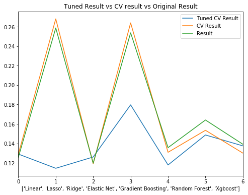
- Hyper Parameter tuned results are much better than original result.
- Regularized linear regression is better than boosting model.
- Best results are Lasso and GBM.
- A little confused that CV result is worse than original result.
- Considering model ensembling / stacking before, but lasso / enet / ridge models are very similar, try simple combination first.
# Lasso Ridge GBM
# m1 = 0.6*lasso + 0.35*gbm + 0.05*ridge
m1 = 0.6*las_mod.fit(x_train,y_train).predict(x_test) + 0.35*gbm_mod.fit(x_train,y_train).predict(x_test) + 0.05*rid_mod.fit(x_train,y_train).predict(x_test)
r = np.sqrt(mean_squared_error(m1,y_test))
print('Combined Model RMSE is : ',r)
Combined Model RMSE is : 0.113704463697
- Simple combined model is better than any single model we have (5%).
- Try stacking model next.
# combined results from 6 single models together
train_index = random.sample(range(1,len(train_data)),round(0.6*len(train_data)))
test_index = random.sample(range(1,len(test)),round(0.6*len(test)))
t_train_stacking = np.vstack(
    (las_mod.fit(train_data.iloc[train_index],train_Price.iloc[train_index]).predict(train_data),
     rid_mod.fit(train_data.iloc[train_index],train_Price.iloc[train_index]).predict(train_data),
     enet_mod.fit(train_data.iloc[train_index],train_Price.iloc[train_index]).predict(train_data),
     gbm_mod.fit(train_data.iloc[train_index],train_Price.iloc[train_index]).predict(train_data),
     rf_mod.fit(train_data.iloc[train_index],train_Price.iloc[train_index]).predict(train_data),
     xgb_mod.fit(train_data.iloc[train_index],train_Price.iloc[train_index]).predict(train_data)))
train_stacking = pd.DataFrame(t_train_stacking.T)
train_stacking.shape
(1458, 6)
# split into train and test part
x_train_stacking,x_test_stacking,y_train_stacking,y_test_stacking = train_test_split(train_stacking,train_Price,
                                                                                    test_size = .3,random_state = 13)
# Using xgb as Level 2 model
l2_mod.fit(x_train_stacking,y_train_stacking)
predictions = l2_mod.predict(x_test_stacking)
print('Level 2 Modeling RMSE Score:',np.sqrt(mean_squared_error(predictions,y_test_stacking)))
Level 2 Modeling RMSE Score: 0.0938204230879
-
Stacking Model result is better than any single model (around 20%).
-
For Further Analysis :
-
1.Covert all numeric variables to dummy variables (1/0)
-
2.Make better Hyper-Parameter-Tuning(Need better computer with more cores).
-
3.Consider other algorithms.
-
4.Set level 3 Stacking.